#statusMessage#
Do you want to start the comparison now?


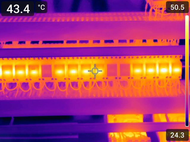
How Thermography Enhances Manufacturing. Machine stoppages, component overheating, or electrical faults—unplanned downti...

Disturbances in the power grid often go unnoticed until systems shut down or equipment fails. Regular power quality asse...

In this practical checklist you will learn how to calibrate your measuring and test instruments effectively – simply, ef...
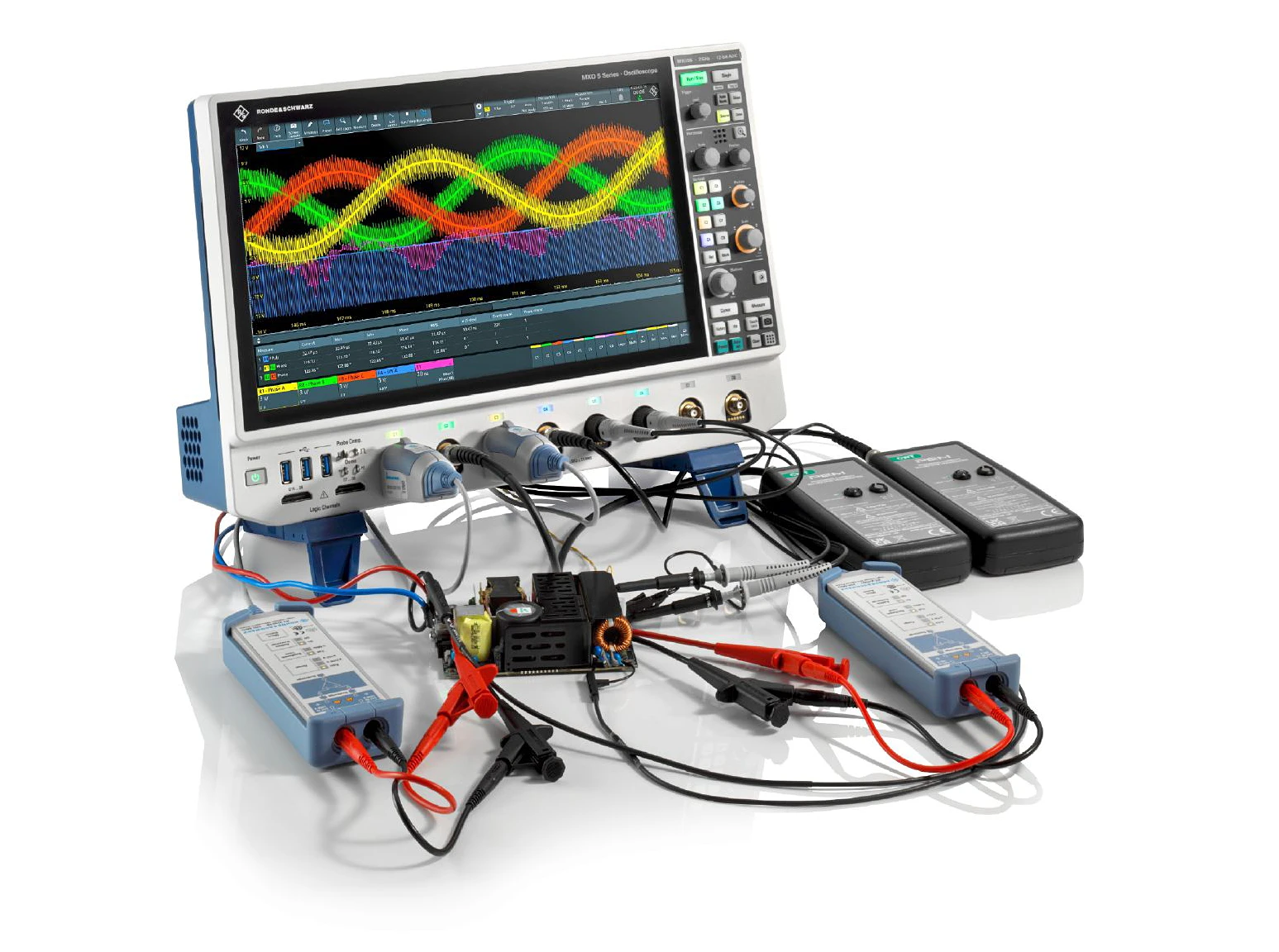
Modern oscilloscopes of the MXO Series from Rohde & Schwarz enable precise analysis and optimization of electric dri...
The market offers a wide choice of oscilloscopes for sale. This makes it difficult to decide which oscilloscope to buy as a new acquisition. This article deals with the most important decision criteria on which a choice can be made.
Decision criteria when buying an oscilloscope include:
Your measurement application defines the technical specifications for the oscilloscope. Depending on the budget, compromises may have to be made when purchasing. However, these compromises should not affect the crucial factors. An oscilloscope can be used to display signals over time. Trigger conditions determine the recording and display of the signals. The two-dimensional display shows the signal amplitudes on the y-axis, while the x-axis shows the time curve.
This leads to five key parameters that influence your choice of oscilloscope:
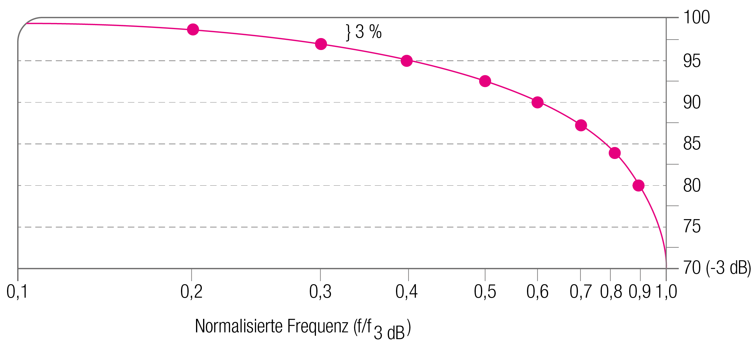
The bandwidth (given in Hz) describes the frequency range over which the oscilloscope can measure. It is defined as the frequency at which a sinusoidal input signal is attenuated to 70.7% of the original signal amplitude. A sine signal with a frequency of f0 and an amplitude of 1 Vpp is therefore displayed as 0.7 Vpp.
This value is also referred to as the -3 dB point or -3 dB limit (see Fig. 1). If the bandwidth is chosen too low, the oscilloscope cannot detect any high-frequency changes. The amplitude may be distorted and the edges are difficult to see, so that signal details are lost.
To determine the optimum oscilloscope bandwidth that allows you to precisely characterize the signal amplitude, the bandwidth of the oscilloscope should be at least five times the highest frequency component to be measured. This means that the oscilloscope is capable of detecting the 5th harmonic of the clock signal and, for example, of displaying a square wave signal as such.
Fig. 1: The oscilloscope bandwidth describes the frequency at which a sinusoidal input signal is attenuated to 70.7% of its original amplitude (also known as the -3 dB limit; in German).
To determine the optimum oscilloscope bandwidth that allows you to precisely characterize the signal amplitude, the bandwidth of the oscilloscope should be at least five times the highest frequency component to be measured. This means that the oscilloscope is capable of detecting the 5th harmonic of the clock signal and, for example, of displaying a square wave signal as such.
In principle, all oscilloscopes have a frequency response like that of a low-pass filter. They differ in how the frequency response drops off from the -3 dB limit. Broadband oscilloscopes (>1 GHz) generally have a steeper drop of 40 dB/decade (see Fig. 2) and can perform much more accurate measurements of the pulse edge steepness within their bandwidth than oscilloscopes with a bandwidth <1 GHz with a drop of 20 dB/decade. Its filter exhibits Gaussian behavior. Regardless of the frequency response of the oscilloscope, the -3 dB point determines its bandwidth by definition (see Fig. 3).
As far as the bandwidth is concerned, note the following points: The measuring system comprises not only the oscilloscope, but usually also a probe. These two together form the relevant system bandwidth. The low-pass filter with the smallest bandwidth ultimately determines the system bandwidth.
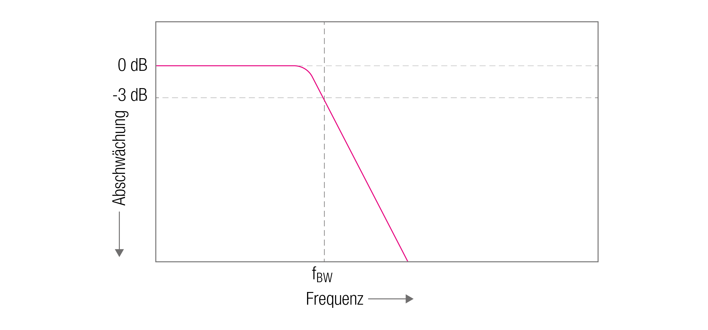
Fig. 2: Typical frequency response of an oscilloscope with a bandwidth >1 GHz (in German)
Fig. 3: Typical frequency response of an oscilloscope with a bandwidth <1 GHz (in German)
The measuring system comprises not only the oscilloscope, but usually also a probe. These two together form the relevant system bandwidth. The low-pass filter with the smallest bandwidth ultimately determines the system bandwidth.
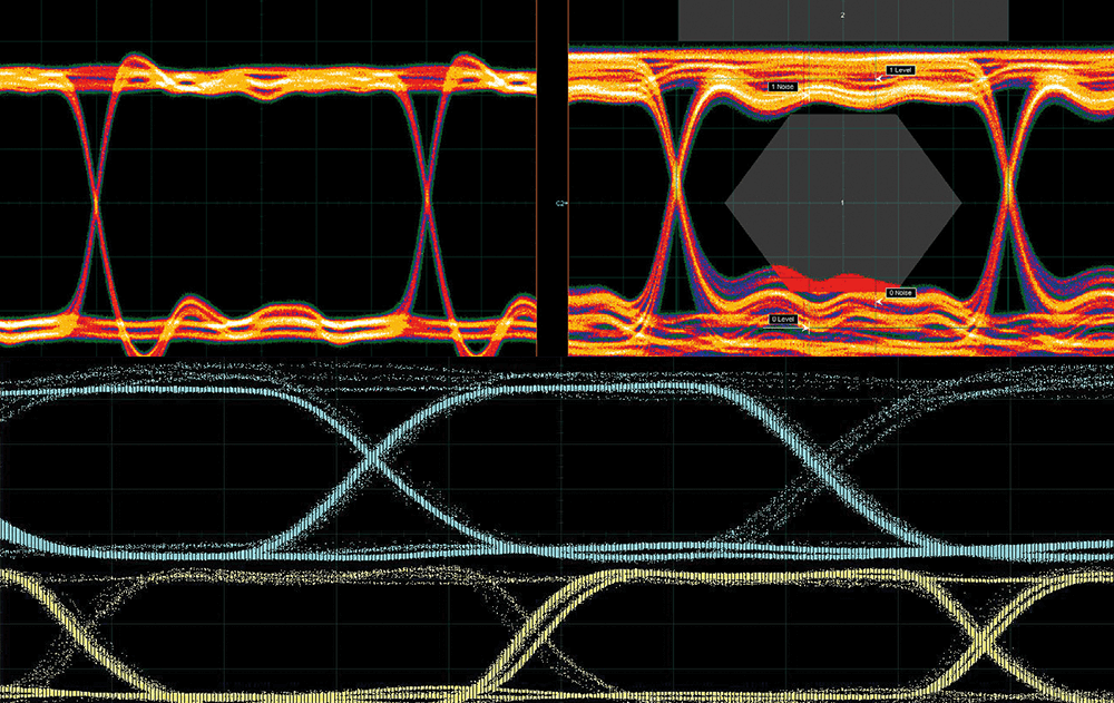
The rise time can be a suitable performance criterion if digital signals, e.g. pulse and step signals, are to be measured. A steep edge is important here (rise time/fall time) so that the receiver can decide between 1 and 0 within the unit interval. For this reason, input filters with a steeper slope (see Fig. 2) are generally used with oscilloscopes with a bandwidth >1 GHz.
The rise time describes the usable frequency range of an oscilloscope. The following equation can be used to calculate the oscilloscope rise time required for a particular type of signal:
The rise time of the input signal is the time that the signal needs for the transition from 10% to 90% of the maximum amplitude (see Fig. 4). The rise time of the oscilloscope should be one third to one fifth of the rise time of the signal to be measured. An oscilloscope with a faster rise time can capture important details of fast transitions more accurately. The relationship between the rise time of the oscilloscope (Tr) and the bandwidth (BW) can be established using the constant "k":
The constant "k" depends on the oscilloscope. For oscilloscopes with a bandwidth of <1 GHz, k = 0.35. For oscilloscopes with a bandwidth of >1 GHz, "k" is typically between 0.4 and 0.45.
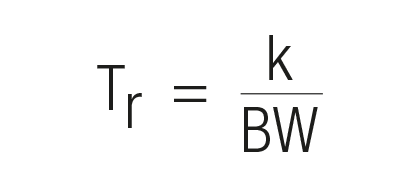
Fig. 4: The rise time (edge steepness) of an input signal is the time it takes for the signal to transition from 10% to 90% of the maximum amplitude.
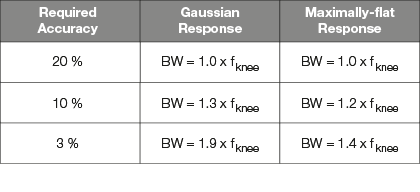
One example: Using an oscilloscope with Gaussian frequency characteristics, a signal with a rise time of 1 ns is to be measured with an accuracy of 3%. With fKnee = 0.5 / 1ns and the table value for the BW = 1.9 * fKnee, this results in a bandwidth of 950 MHz. Accordingly, an oscilloscope with a bandwidth of 1 GHz is selected. The clock rate of the digital signal, whether 100 or 500 MHz, is not relevant here; the rise time determines the required bandwidth.
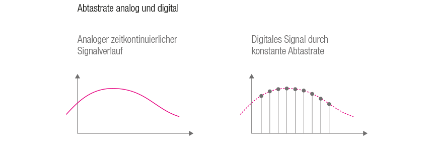
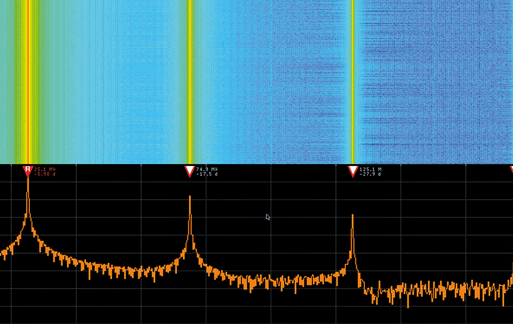
The sample rate (Sa/s, samples per second) is the frequency at which the A/D converter converts the analog signal input values into digital data. The oscilloscope samples the input signal after attenuation, amplification or filtering has been applied to the analog input path. The higher the sample rate, the better the temporal resolution and thus the details that can be recognized in the signal curve. The "Nyquist sampling theorem" explains the relationship between the sample rate and the frequency of the measured signal. It states that the sample rate fs must be at least twice as high as the highest frequency component to be analyzed in the measured signal (also known as the Nyquist frequency) in order to represent it unambiguously.
Real-time sampling is an ideal sampling mode for signals whose frequency range is less than half the maximum sample rate of the oscilloscope, e.g. to capture fast, one-off, transient signals (Figure in German).
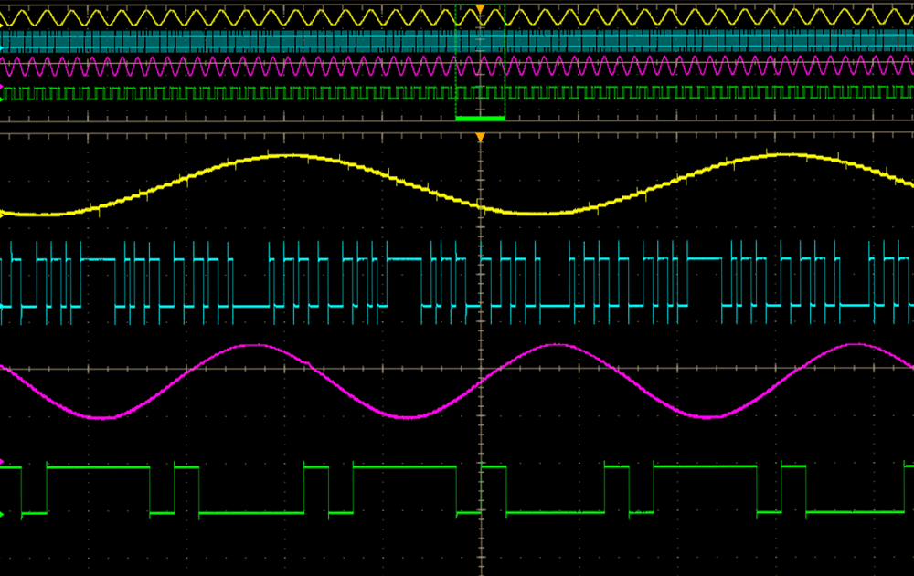
Most oscilloscopes can measure several signals simultaneously and display them on the screen. Each individual signal recorded by an oscilloscope is fed into a separate channel. Models with two, four or even eight channels for analog signals are common.
Mixed-signal oscilloscopes (MSO) usually also have eight or 16 digital inputs for displaying and analyzing time-correlated analog and digital signals. As logic analyzers, these channels can decode digital signals - including serial signals - and display them in the appropriate mask field in accordance with the standard. Signal anomalies and errors can thus be easily detected.
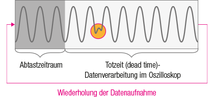
The signal acquisition rate indicates how often the complete displayed signal or a signal section is acquired per second (given in wfms/s, waveforms per second). The number of acquisitions depends, among other things, on the set time resolution (seconds per scale division, e.g. ns/div) and the memory depth for saving the acquired signal sequences. An oscilloscope requires a time X after each sampling cycle of an incoming signal in order to process the data (storage and display on the screen). The shorter this processing time (dead time) is, the faster the oscilloscope samples a new signal and can therefore, for example, also detect sporadic signal anomalies more quickly (see Fig. 4).
With multi-channel oscilloscopes, the sample rate and signal acquisition rate may be reduced if several channels are in use. This depends on how the internal storage process is implemented. The sample rate and signal acquisition rate often adapt automatically to the storage conditions.
Fig. 6: Sample rate, signal acquisition rate and memory depth are interrelated. Signal anomalies can remain hidden if the signal acquisition rate (wfms/s) is too low (in German).
The number of scans is limited by the memory depth: In order to be able to use the maximum sample rate for a longer period of time, a deep memory is required. The memory requirement is calculated using a simple formula based on the longest time range setting required and the maximum sample rate at which you want to record a signal: Storage depth = recording duration * sample rate. However, this only applies if each input channel of the oscilloscope has the same memory depth. The recording duration is usually adjustable in order to achieve optimum and detailed recording of signals.
Note: In the case of sporadic signal events, it is advantageous to have the deepest possible memory and a high signal acquisition rate in order to be able to store as many signal sequences as possible.
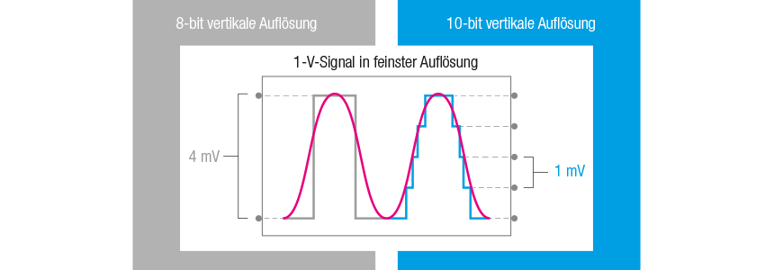
The vertical resolution of a digital oscilloscope indicates the accuracy with which the A/D converter converts the input voltage into digital values. Eight to 16 bits are common.
Example: An oscilloscope with a resolution of 10 bits achieves 1024 measurement points in the vertical plane. With the setting "1 volt per scale division" with 10 screen scale divisions in the y-direction, 10 volts ("full deflection") can be measured. With a resolution of the A/D converter of 1024 points, this means that a measurement point is set on the screen at intervals of 9.76 mV. With modern oscilloscopes with 16-bit resolution, the measurement points in the above example are even taken every 0.153 mV.
The effective amplitude resolution of some oscilloscopes can also be increased using digital calculation methods, e.g. in high-resolution acquisition mode (Hi-Res mode, HD mode), (Figure in German).
The evaluation of your measurement results is just as important as the efficient exchange of information and reliable documentation. The connectivity of your oscilloscope, e.g. via USB, RS-232, LAN, WLAN or Bluetooth, enables extended analysis functions and simplifies the documentation and exchange of results. In addition, your measuring devices can be integrated into networks via appropriate interfaces and controlled remotely via the web.
Triggers are used to stabilize repetitive signals on the screen, to capture single-shot signals or to mark a specific point of a capture. The trigger functions of an oscilloscope synchronize the horizontal deflection at the correct signal point, which can be crucial for clear signal characterization.
Your oscilloscope should also be able to meet future, changing measurement requirements in order to be economical. Corresponding oscilloscopes allow the number of channels, bandwidth or memory depth to be expanded at a later date. Software options, e.g. math functions, FFT (Fast Fourier Transformation) or masks for standard transmission protocols, can be used to add application-specific measurement functions and extend the performance and functionality of the device: e.g. with an integrated digital voltmeter, frequency meter, power meter, arbitrary function generator or spectrum analyzer. Oscilloscopes can also be supplemented by a comprehensive selection of probes, clip-on ammeters and application modules.
The digital storage oscilloscope is a conventional digital oscilloscope. It enables the recording and display of one-off events, so-called transients. DSOs use a serial processing architecture for this purpose. The signals can be documented and analyzed on the oscilloscope itself or on an external PC. A DSO offers permanent signal storage and comprehensive signal processing.
Keysight | Tektronix | Rohde & Schwarz | Pico Technology | GW Instek
The mixed-signal oscilloscope combines the measurement and analysis functions of a DPO with the basic functions of a 16-channel logic analyzer, including the decoding and triggering of parallel and serial bus protocols. The digital channels of the MSO use a threshold voltage to determine whether the signal level is logic high or logic low, just as a digital circuit recognizes the signal. With its powerful digital triggering, high-resolution acquisition and analysis tools, the MSO is ideal for fast troubleshooting of digital circuits by analyzing both the analog and digital signal representation.
Keysight | Tektronix | Rohde & Schwarz | Pico Technology | GW Instek
Digital phosphor oscilloscopes use a parallel processing architecture with high signal acquisition rates to display and analyze a signal. With their capabilities, signals can be reconstructed precisely. Compared to a DSO, DPOs can better detect transient events in digital systems, e.g. runt pulses, glitches or edge errors, and also offer extended analysis options.
Tektronix
A mixed-domain oscilloscope combines an MSO or DPO with the capabilities of a spectrum analyzer. It provides a time-correlated representation of protocol, state logic, analog and RF signals within an embedded system, significantly speeding up troubleshooting. It also reduces measurement uncertainties for cross-range events. If the time delay between a microprocessor command and an RF event can be tracked within a system, this simplifies the test configuration and enables complex laboratory measurements.
Tektronix | GW Instek
In the architecture of a digital sampling oscilloscope, the positions of the attenuator or amplifier and sampling bridge are reversed compared to the DSO/DPO architecture. The input signal is therefore sampled before the attenuation/amplification and converted to a lower frequency. This results in a measuring device with a very high bandwidth. The disadvantage is the limited dynamic range of the sampling oscilloscope. In addition, protection diodes cannot be used upline of the sampling bridge as this would limit the bandwidth, reducing the safe input voltage of a sampling oscilloscope to around 3 V compared to 500 V for other types of oscilloscope.
The equivalent time sampling method of the digital sampling oscilloscope is ideal for the precise acquisition of high-frequency, repetitive signals whose frequency components are significantly higher than the sample rate of the oscilloscope.
Tektronix | Pico Technology
During sampling, part of the input signal is converted into a series of discrete electrical values. The value of the displayed sampling points corresponds to the amplitude of the input signal at the time of sampling. Each snapshot therefore corresponds to a specific point in time in the signal. The digital oscilloscope displays a series of sampling points with the measured amplitude on the vertical axis and the time on the horizontal axis, thus reconstructing the input signal. A distinction is made between a real-time oscilloscope and an equivalent time oscilloscope (sampling oscilloscope). Some oscilloscopes offer a choice of sampling method: real-time sampling or equivalent time sampling.
With high-frequency signals, DSO or DOP may not be able to detect enough sampling points during a deflection. The equivalent time sampling of a digital sampling oscilloscope enables the exact acquisition of signals whose frequency components are significantly faster than the sample rate of the oscilloscope. Repetitive signals can be reconstructed by capturing a small amount of information with each repetition.
There are two types of equivalent time sampling methods: random and sequential. Both methods require a repetitive input signal. With random equivalent time sampling, the sampling is asynchronous to the input signal and signal trigger. This enables the input signal to be displayed before the trigger point; external pre-trigger signals or delay lines are not required. With sequential equivalent time scanning, a single scan is performed for each detected trigger after a defined time delay. When the next trigger occurs, this delay is increased. Sequential equivalent time sampling offers significantly higher temporal resolution and accuracy.
Real-time sampling is ideal for signals whose frequency range is less than half the maximum sample rate of the oscilloscope. A real-time oscilloscope can also be used to record one-off or sporadically occurring transient signals. This requires a very high sample rate. In the event of under-sampling, the high-frequency components can be "folded" into a lower frequency and cause aliasing effects in the display. In addition, real-time sampling requires a high memory depth in order to store the signals after digitization.
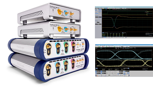
USB digital oscilloscopes, e.g. from Pico Technology, require a USB connection to an external PC and associated software applications to control the oscilloscope and display measurement curves. The devices, virtually the front end of conventional laboratory oscilloscopes, are particularly light and compact and therefore ideal for mobile use and service applications. USB sampling oscilloscopes and USB real-time oscilloscopes are available on the market.
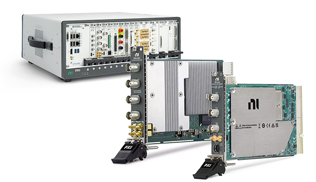
The PXI test system from NI includes powerful, modular measurement devices and input/output modules that have special software and synchronization functions. The system is particularly suitable for test applications with a high number of channels, for production tests in automated manufacturing and for device validation. A PXI system consists of three hardware components: Chassis, controller and peripheral modules. The NI portfolio comprises over 600 PXI modules for data acquisition, control and regulation, including modular measuring devices such as oscilloscopes. The oscilloscope modules can be integrated into the PXI hardware platform and replace conventional desktop devices. PXI oscilloscopes are flexible, software-defined measuring devices. They offer users the benefits of the powerful, scalable, industry-standard PXI platform. The PXI platform allows multiple oscilloscopes to be synchronized with other measuring devices with picosecond accuracy.
You are not quite sure yet or have further questions about the products? Do not hesitate to contact us. Whether directly on the phone or via online demo conveniently in front of your screen - our experts are there for you.


